Lab Manual
Contents
Table of Contents
Introduction: Electrical Circuit Models of Membrane Properties
Today you will use electrical circuit models of a passive cell membrane to introduce yourself to some of the basic components of your essential electrophysiology toolkit. You will interrogate some of the passive properties of neural membranes and compare the difference between membrane potential “spikes” recorded intracellularly and membrane potentials recorded extracellularly.
This module will help you work on:
Describing passive properties of neural membranes that critically affect neural processing.
Using a voltage meter.
Relating basic electrical circuit components to fundamental physiological properties of neurons (Resistance, Capacitance, Serial, Parallel, Voltage, Current).
Storing, managing, and visualizing data on the computer.
Creating figures that summarize your data and analysis - enabling you to discuss your results.
Electrical Circuit Components
A small set of electrical components can be used to describe many of the basic electrophysiological properties of neurons.

Resistors are electrical components that resist the flow of current through a circuit. The amount of current flowing through a resistor can be expressed by Ohm’s Law: \(I = V/R\), where I represents the current, V represents the voltage, and R represents the resistance. Similarly, \(V = IR\) determines the voltage in response to a current across a resistor.
In an electrical circuit, a capacitor possesses two conducting regions with a separation of non-conducting material in between. When one conducting region accumulates a charge (due to current flow from an external voltage source), an electric field is created, which pushes the charge off of the subsequent conducting region of the capacitor. This phenomenon only lasts a short amount of time, producing a brief current which is expressed as: \(I = C * \partial{V}/\partial{t}\), where \(I\) represents the current, \(C\) represents the capacitance, and \(\partial{V}/\partial{t}\) represents the rate of voltage change with time. Current flows across the membrane capacitance only when voltage across the membrane changes.
Since the lipid bilayer is an electrical insulator between two conducting areas (extra- and intracellular fluids), it acts as a capacitor, while ion channels act as resistors. Membrane capacitance is parallel to membrane resistance (though a circuit in series can be equivalent for some purposes).
Electrical Circuit Models
Membrane potentials
This model simulates how the interaction among ionic conductances controls the membrane potential.

For example, in this model, \(R_K\) is the resistance through potassium channels, \(R_{Na}\) is the resistance through sodium channels, and \(C\) is the capacitance of the lipid bilayer (not necessary for understanding steady state properties). By convension, we measure the inside of a neuron’s membrane with respect to the outside (“ground”).
Passive spread
This model simulates a cylinder-like compartment of a neuron, such as an axon.

In this lab, the circuit you will use for this model has the following \(R\) values:
Rinside = 1 kOhm
Routside = 100 Ohm
Rmembrane = 10 kOhm
Note that resistances in parallel sum according to \(1/R_{total} = 1/R + 1/R + ...n \) while resistances in series sum according to \(R_{total} = R + R + R + ...n\).
Membrane response dynamics
This model summarizes the entire membrane of the neuron into a single compartment/point to examine how resistive and capacitive properties effect how neurons respond to inward/outward current (for example synaptic events).

In this lab, you will start with values of \(R=10MOhm\) and \(C=0.001uF\).
Setup
Physical Rig Hardware Setup
You will be using An analog to digital converter (ADC; the NiUSB-6211 from National Instruments) to measure the ‘membrane potential” in your model circuits for Parts I-III. An ADC digitizes the analog voltage input and sends it to the computer for visualization and recording of the raw (digitized) data. The electrode wires connect directly into the input of the NiDAQ ADC.
Physical Rig Software Setup
Bonsai-rx is an open-source software for managing streems of data from devices on a computer. Open the bonsai workflow (passive-membrane-models.bonsai) from the Documents/BIOL247/data/passive-membrane-models folder on the lab PC.
Modify the sampling rate of Analog-to-Digital conversion (ADC rate) by clicking on the Analog Input node. Make sure that the sampling rate is set to 10kHz for this lab and the Analog Input range is -10 to 10 V.
Whenever you want to visualize the electrode measurements without accumulating stored data on the PC harddrive, just disable the Matrix Writer node. You can specify a filename for your data by clicking on the Matrix Writer node and enable it to record your data to disk. By default, files are saved in the same folder as the bonsai workflow file.
Hitting the start button on the workflow will start the digitization of data from the NiUSB.
Double-clicking on the Select Channels nodes will enable you to visualize a live stream of the raw data from the electrodes.
Python Notebook Setup
#@title {display-mode:"form"}

#@title Run this cell to initialize packages and functions

from pathlib import Path
import numpy as np
import matplotlib.pyplot as plt
import plotly.graph_objects as go
from plotly.subplots import make_subplots
from ipywidgets import interactive, HBox, VBox, widgets, interact
Part I. Membrane Potential
You will create the following circuit (ignoring capacitance) on a breadboard.
Setup:
Use one battery for \(E_K\) and one battery for \(E_{Na}\) (make sure to measure and record the voltage of each battery… you will also use this info in future labs)
Start with equal resistors for \(R_K\) and \(R_{Na}\) (make sure to measure and record the value of each resistor… you will also use this info in future labs).
Place the recording/measuring electrode on the ‘inside’ of the membrane
Place the ground electrode on the ‘outside’
In the Bonsai workflow, Disable the “Matrix Writer” node.
Experiment:
Hit play in Bonsai. Double click on the “Membrane Potential” node if the window is not already present. Close the “Stimulus” window if it is open.
Right mouse click on the bottom of the membrane potential window to change the y axis range of the graph as needed.
Hover over the signal trace with your mouse to see the voltage. Record the measured ‘membrane’ potential of the model cell along with the model cell \(C\) and \(R\) and \(E\) values (and their organization).
Note that membrane potential is measured inside the cell relative to outside and the Getting amplifier has a gain of 10.
Keeping \(R_K\) constant, change \(R_{Na}\) and record the measured ‘membrane’ potential. (make sure to measure and record the value of each electrical component… you will also use this info in future labs)
Keeping \(R_{Na}\) constant, change \(R_K\) and record the measured ‘membrane’ potential. (make sure to measure and record the value of each electrical component… you will also use this info in future labs)
Keeping \(R_K\) and \(R_{Na}\) constant, change the polarity of one or both batteries and record what happens to the measured ‘membrane’ potential with each change in polarity configuration.
Stop the data acquisition by hitting the stop button in Bonsai.
Part II. Intracellular Recording of Applied Voltage
You will use the following passive axon model (pre-made) to complete this experiment. The axon model has 13 total nodes rather than the 3 shown here.
Setup:
At the middle of the axon (node 5), place one electrode on the ‘inside’ of the membrane and one on the ‘outside’.
Note that membrane potential is measured inside the cell relative to outside.
In Bonsai, Disable the “Matrix Writer” node.
Experiment:
Attach a voltage source (battery) across the cell membrane at the end of the axon (node 0). The positive lead of the voltage source should go inside the membrane, and the negative lead should go outside.
Move the voltage source along the axon one node at a time until you reach node 10.
At each node, record the voltage in the dictionary below by replacing the
...with the measured value.
Note that the Getting amplifier has a gain of 10.
voltage_intracellular = {
    '0' : ...,
    '1' : ...,
    '2' : ...,
    '3' : ...,
    '4' : ...,
    '5' : ...,
    '6' : ...,
    '7' : ...,
    '8' : ...,
    '9' : ...,
    '10' : ...
}
Run the code cell in which you just defined your data dictionary.
Then, run the following code cell to plot your data.
#@title {display-mode:"form"}

#@markdown Run to plot data.

nodes = list(map(int, list(voltage_intracellular.keys())))
voltage = list(voltage_intracellular.values())

plt.figure()
plt.plot(nodes,voltage)
Part III. Extracellular Recording of Applied Voltage
Use the same passive axon model that you used in Part II and a voltmeter to complete this experiment.
Setup:
At the middle of the axon, place both electrodes on the ‘outside’ of the membrane, with one empty node between them (one electrode at node 4 and one at node 6).
In Bonsai, Disable the “Matrix Writer” node.
Experiment:
Attach a voltage source (battery) across the cell membrane at the end of the axon (node 0). The positive lead of the voltage source should go inside the membrane, and the negative lead should go outside.
Move the voltage source along the axon one node at a time until you reach node 10.
At each node, record the voltage in the dictionary below by replacing the
...with the measured value.
Note that the Getting amplifier has a gain of 10.
voltage_extracellular = {
    '0' : ...,
    '1' : ...,
    '2' : ...,
    '3' : ...,
    '4' : ...,
    '5' : ...,
    '6' : ...,
    '7' : ...,
    '8' : ...,
    '9' : ...,
    '10' : ...
}
Run the code cell in which you just defined your data dictionary.
Then, run the following code cell to plot your data.
#@title {display-mode:"form"}

#@markdown Run to plot data.

nodes = list(map(int, list(voltage_extracellular.keys())))
voltage = list(voltage_extracellular.values())

plt.figure()
plt.plot(nodes,voltage)
Part IV. Membrane Potential Dynamics with Applied Current
For this exercise, you will use the following passive resistor-capacitor circuit model membrane.
You will be using the Getting Intracellular Amplifier to both deliver current and measure voltage. The Getting provides a current stimulation, feature that applies a “square wave” stimulus across the measurement electrodes. A square wave stimulus one that instantaneously increases in amplitude and maintains that amplitude some duration before instantaneously decreasing to 0.
The Getting accepts an externally-controlled square wave stimulus through the STIM. INPUTS BNC on the front panel. This allows more precise control over the pulse duration, timing, and amplitude by using a pulse generator (“stimulator”). There are three different stimulator models currently available in the lab, that each have similar functionality, but different controls. They are all called Stimulus Isolating Units (SIU). The two SIUs that are at the rigs for today are the Grass SD-9 and the AM-Systems.

Setup:
Create the circuit depicted in the circuit diagram above. Start with Resistance = 5 MOhm and a “103” capacitor.
Place the recording/measuring electrode on the ‘inside’ of the membrane
Place the ground electrode on the ‘outside’
If you are using a separate SIU and amplifier, set up the stimulus electrodes so that you can “apply” current into the model membrane (one stimulating electrode on the outside and one on the inside). You will need to use a model circuit in series rather than parallel so the recording does not short the stim.
In Bonsai, Disable the “Matrix Writer” node.
Hit play. Double click on the Select Channels nodes to visualize the input from the Amplifier Output and Stim Monitor if the windows are not already present. Make sure that you see a signal on both channels. Adjust the y-axis range: stimulus monitor (-0.5,1.1) and membrane potential (-0.5,1.1). If the membrane potential is not visible, adjust the y-axis range so that you can see where the signal offset is, and then use the POSITION knob on the amplifier to get the DC offset of the amplifier back in range.
Note that a copy of the stimulus (current monitor) is being sent to the NiUSB ADC. The coversion factor is 100 mV per nA.
Note that the Getting Amplifier has a gain of 10X on the membrane measurement.
Experiment
Baseline Configuration
Set the SIU to 500ms duration at approximately 0.5Hz and 500 milliVolts.
Enable the “Matrix Writer” node.
Turn the SIU to repeat until 3 stimulus pulses have completed.
Stop the data acquisition by hitting the stop button in Bonsai.
Change Resistance
Increase Resistance relative to #1
Record and repeat Stimulation protocol
Decrease Resistancerelative to #1
Record and repeat Stimulation protocol
Change Capacitance
Return to a resistance of 5 MOhm
Increase capacitance to a 104
Record and repeat Stimulation protocol
Decrease capacitance to a 102
Record and repeat Stimulation protocol
Upload your data files to an external drive OR to your Google Drive.
Use the DataExplorer.py application found in the How To section of the course website to explore and analyze your data.
Stop here for a class discussion about what you notice from this final experiment and a tutorial on the DataExplorer.py application.
Experiment extensions (time permitting):
What happens when you change the stimulus amplitude?
What happens when you change the stimulus duration?
What happens when you change the resistance of the model cell?
What happens when you change the capacitance of the model cell?
Housekeeping
Clean up your area.
Copy data to an external drive or your Google Drive for later.
Use the DataExplorer.py application to explore your raw data in detail. Answer the questions in the Responses notebook.
Additional Resources
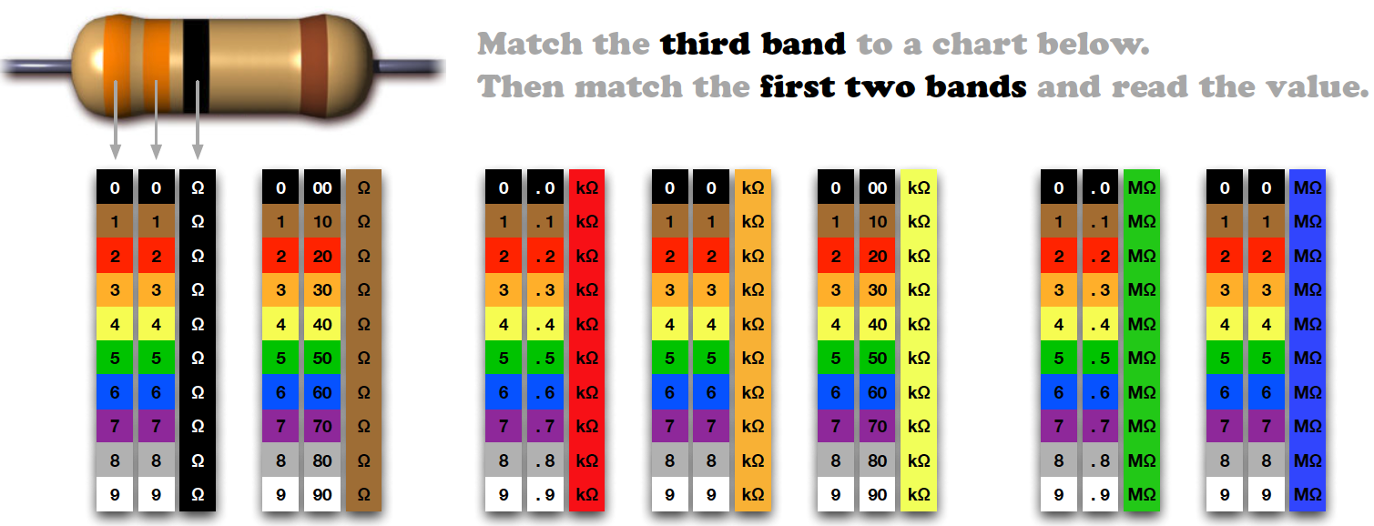
Resistor Decoder
From worrydream
Written by Dr. Krista Perks for courses taught at Wesleyan University. Materials based off of William Kristan's graduate student bootcamp at UCSD and the Membrane Properties Lab in the Crawdad Lab Manual by Robert A. Wyttenbach, Bruce R. Johnson, and Ronald R. Hoy